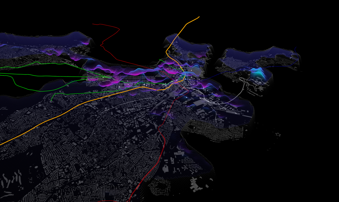
Trajectory data, which records locations of moving objects at certain moments is an interesting means of studying mobility behaviour. Trajectory data analysis is of significant practical value and there are numerous applications and services of trajectory data for the government, commercial organizations, and individuals[3]. Public transport services like busses and taxis are vital for general public commuting and are often equipped with GPS location devices. These GPS devices record data providing us with a digital footprint of individual mobility patterns. Such historical data, if analysed, contains potentially valuable insights for the identification, addressing and optimization of urban road network related problems.
In this Project, we analyse the CRAWDAD roma taxi driver dataset for possible cases of fraud. A taxi driver sometimes tries to maximize his income using unethical ways(taking longer route where a shorter one exists). Our goal is to find cases in which taxi drivers drive from one location to another location that is neither the shortest distance route and nor the fastest route(exception is the traffic jams where one is allowed to take an acceptable slightly longer alternative if available). We call such cases “fraud”. The problem of picking good routes is studied well in literature and is known as Taxi Driver's Mobility intelligence[1].
Trajectory data:
This dataset contains mobility traces of taxi cabs operating in metropolitan city of Rome, Italy. It contains GPS coordinates of approximately 320 taxis collected over 30 days. Data was collected during the period from 01/Feb/2014 until 02/March/2014 and it represents drivers who work in the centre of Rome. The data can be downloaded from this website, and comes in CSV format.
The question we seek to answer is:
- Can fraudulent behaviour be inferred from the trajectories implicitly given in the dataset(described below). i.e Are some drivers more likely to commit fraud than others? If yes how can we count the suspect cases?
- How common is fraud among the various drivers?
This problem is challenging because the dataset has limitations. For starters, since start and end points of the journey's are not provided, we will have to figure out a way by which we can identify the starting point and the end point of a journey. Secondly, we will have identify some of the the sensible routes (ones that are optimal in the sense of being shortest or fastest) and then compare a typical route taken by taxi drivers to those optimal routes. Lastly, this is a big dataset and at the time of analysis currently popular libraries don't support loading the full dataset into the memory so we will have to look for alternate methods.
Loading the data
Upon doing a bit of trial and testing, it was found that fread is the fastest method to load large datasets(especially on machines with limited memory):
#load data install.packages("data.table")
library(data.table)
taxi_data = fread(file.choose(), header = T, sep = ',',data.table=FALSE)
Exploring the data:
After loading the dataset, we perform a general exploratory analysis of this dataset to understand the data at hand.
Here is a quick peek:

The dataset contains 4 attributes:
- ID of a taxi driver. This is a unique numeric ID.
- Date and time in the format Y:m:d H:m:s.msec+tz, where msec is micro-seconds, and tz is a time-zone adjustment.
- Longitude, Latitude: These provide explicit trajectory information and if analysed properly contains rich spatiotemporal information.
Since they are a a series of chronologically ordered points, they represent taxi movement traces. i.e spatial trajectory generated by moving taxis in Rome.
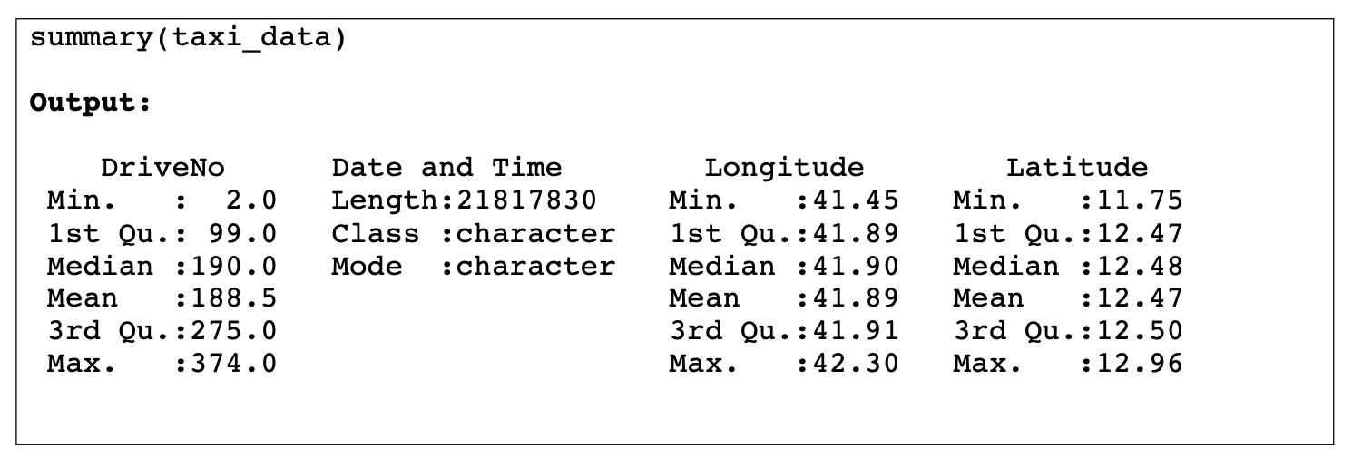
In exploratory phase, a good way to start is to get a high level overview of the data using the summary method, which shows the relevant stats such as the total number of samples, possible missing values and the data type for each column. Let's get compute some quick stats(minimum, maximum, and mean location values)
Visualisation:
Visualisation is an effective way to understand the data at hand and get a sense of common routes taken by the taxi drivers. Since we are plotting 27 million rows of data, the basic plot will get us nothing but a splash of circles on the screen. We experimeted with ggplot and its size parameter to obtain a sensible. (this also saves compute time).
#Plot the location points (2D plot)
#create a dataframe

taxi_pickup_data <- data.frame(taxi_data[,.(Longitude)], taxi_data[,.(Latitude)])
taxi_pickup_data <- data.frame(taxi_data[,.(DriveNo)], taxi_data[,.(DateandTime)])

#basic plot gives a big blob (uncomment if needed)
#plot(taxi_pickup_data)


install.packages("ggplot2")
library(ggplot2)

ggplot(taxi_data, aes(x= Longitude, y= Latitude)) + geom_point(size=0.02)
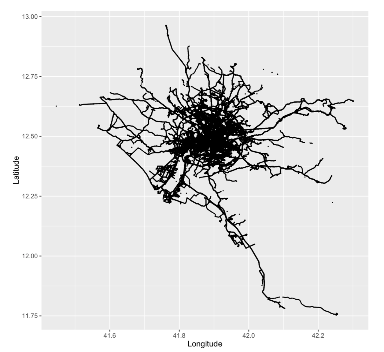
This doesn't make a lot of sense but we can clearly see some points are not part of the trips(outliers). Let's proceed to pre-processing and come back to improving the plot later.
Pre-Processing:
In this step we identify missing values, erroneous entries and remove a few outliers(noise or data that is not relevant to our analysis)
remove duplicates:
taxi_data_subset = taxi_data_subset[!duplicated(taxi_data_subset[1:3]), ]Detecting outliers:
Easiest way to remove outliers is to simply plot the longitude and latitude and visually define the area of Rome on which we want to focus our analysis.
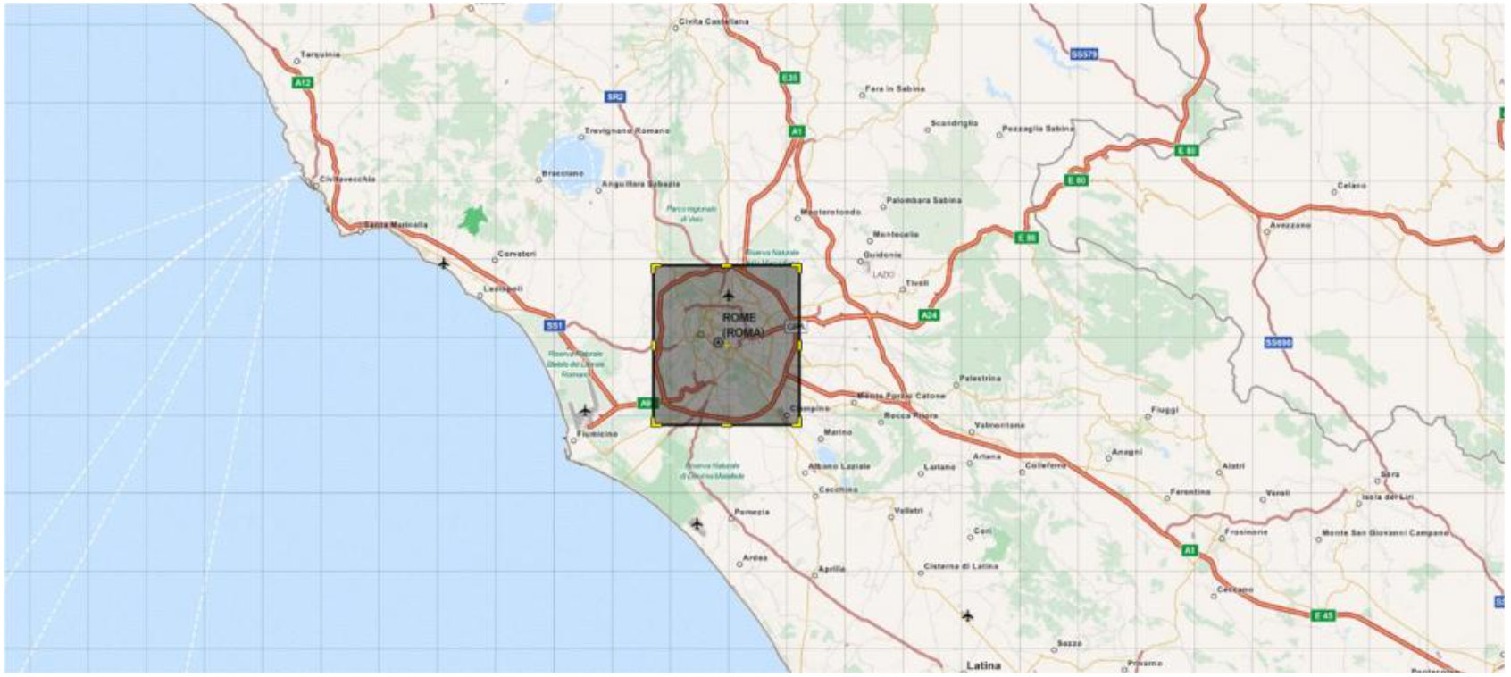
A bounding box was created(as shown in Figure 1) with the below values. The bounding box is based on rome city coordinates from google maps.
Any point outside this bounding box was considered an outlier as it was too far from the heart of the city.
Min_lat= 41.793710
Max_lat = 41.991390
Min_lon = 12.372598
Max_lon = 12.622537
we will create a Tranformation Function for preprocessing and applying Tranformation to raw data.
nw <- list(lat = 40.5, lon = 13)
se <- list(lat = 43, lon = 11)


trans <- function(x) {
    # set coordinates outside of NYC bounding box to NA
   ind <- which(x$Longitude < nw$lon & x$Longitude > se$lon)
   x$dropoff_longitude[ind] <- NA
   ind <- which(x$Longitude < nw$lon & x$Longitude > se$lon)
   x$Longitude[ind] <- NA

 }

#Apply the Tranformation
taxi_data_subset = trans(taxi_data_subset)
The result of applying the bounding box was that 1,563,893 points were removed as outliers.
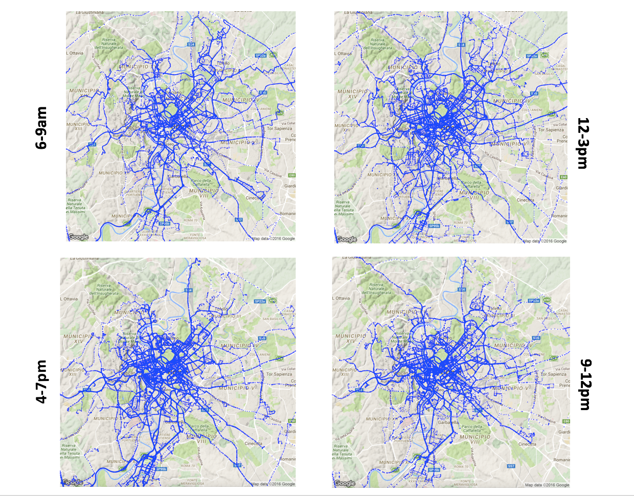
Now with the relatively clean dataset, we can give visualisation and EDA another shot. For dataset to make more sense, we can visualize the dataset on top of the rome's actual map. We can confirm from the figure below that city centre are the frequently visited regions of rome. We can also see how timings effect the routes as many of the trips early in the day and late afternoon could be part of the daily commute for taxi customers.
Analysis of Travel Behaviour:
We can Obtain the most active, least active, and average activity of the taxi drivers (most time driven, least time driven, and mean time driven)
Identify the most Active drivers:
Most active drivers earn the most revenue and chances are they will be following the most optimal routes instead of engaging in fraudulent behaviour. Let's calculate taxi activity is to compute total time driven by each taxi driver
compute_timedriven_2 <- function(DriverID,mytaxi_data) {
print("calculating total_time for driver no.")
print(DriverID)


#create a dataframe containing only the rows of that taxi driver and selecting DriveNo and Data and Time Columns only

temp_dataf <- mytaxi_data[mytaxi_data$DriveNo == DriverID,2]
print(summary(temp_dataf))

if(length(temp_dataf) == 0){ return(0)
}

#iterate over the rows total_time <- as.numeric(1.0000)
len = length(temp_dataf) -1 for(i in 1:len){

total_time = total_time + as.numeric(difftime(strptime(temp_dataf[i+1],"%Y-%m-%d %H:%M:%OS"),strptime(temp_dataf[i],"%Y-%m-%d %H:%M:%OS"),units="min"))
}

print(total_time) #return(as.numeric(total_time), digits=15)
}
total_time_driven <- 0.0000 time_driven_list <- list()

for (i in 1:320){
time_driven_list[i] <- compute_timedriven_2(as.double(i),taxi_data_subset) total_time_driven <- total_time_driven + as.numeric(time_driven_list[i])
}
print(which.max(time_driven_list)) print(which.min(time_driven_list))
#average time driven print(as.numeric(total_time_driven/320),digits = 5)
we can repurpose this to compute to the time for any given driver.
compute_timedriven_2 <- function(DriverID,mytaxi_data) {
print("calculating total_time for driver no.")
print(DriverID)

#create a dataframe containing only the rows of that taxi driver and selecting DriveNo and Data and Time Columns only

temp_dataf <- mytaxi_data[mytaxi_data$DriveNo == DriverID,2]
print(summary(temp_dataf))

if(length(temp_dataf) == 0){ return(0)

}
#iterate over the rows total_time <- as.numeric(1.0000)
len = length(temp_dataf) -1 for(i in 1:len){
total_time = total_time + as.numeric(difftime(strptime(temp_dataf[i+1],"%Y-%m-%d %H:%M:%OS"),strptime(temp_dataf[i],"%Y-%m-%d %H:%M:%OS"),units="min"))
}
print(total_time) }
compute_timedriven_2(211,taxi_data)
Similarly, we can write another function that lets us compute the total distance travelled by a particular diver:
compute_distance_travelled <- function(DriverID,taxi_data) {
#create a dataframe containing only the rows of that taxi driver temp_dataf <- taxi_data[taxi_data$DriveNo == DriverID,3:4]
print(temp_dataf)
#radius of earth
R=6371000
distance = 0
total_distance = 0 #print(summary(temp_dataf))
len = length(temp_dataf) -1 for(i in 1:len) {
lon1<- temp_dataf[i,1] lon2 <- temp_dataf[i+1,1]
lat1<- temp_dataf[i,2] lat2 <- temp_dataf[i+1,2]
dlon = lon2 - lon1 dlat = lat2 - lat1
print(dlon) print(dlat)
a = (sin(dlat/2))^2 + cos(lat1) * cos(lat2) * (sin(dlon/2))^2 c = 2 * atan2( sqrt(a), sqrt(1-a))
distance = R * c
total_distance = total_distance + distance

} return(total_distance)
} compute_distance_travelled(122,taxi_data_subset)
These are useful functions that come in handy later for driver comparisons and sanity checks. e.g we can also use to quickly compute a histogram of time travelled for all drivers.
Using these functions, we were able to compute the following stats:
- Most time driven = 941027 seconds(approx. 261.4 hours)
- Least time driven = 753.979 seconds(0.21 hours)
- Mean time driven = 558808 seconds (approx. 155.22 hours)
- Driver 204 drove for a total of 669980 seconds(approx. 186.11 hours). This is more than the average value of the time driven. It falls in the 3rd quartile of time driven.
We can identify top 10 drivers this way and see if their routes are optimal(a baseline could be google map timings). But since the dataset doesn't give start or end journey location co-ordinates, we will first have to figure out a way to extract various routes.
Route Identification:
Since the dataset doesn’t specify starting and ending points of the routes, one of the important tasks in our analysis is to identify driver routes.
Firstly, we have to identify if the driver is on duty or inactive. We use the time filter for doing so. e.g An hour was used as the limiter for deciding if the taxi was on duty or not. If there was a gap of more than an hour between the two GPS points then the time between them will not be considered as part of the total time driven for that driver.
Secondly we assume that Taxi drivers prefer to roam around the areas with the most potential customers which would mean we should find that many journeys would begin or end at destinations like railway stations, hotels and other places of interest for visitors.
One way to approach this is to use GPS co-ordinates of popular destinations(using google maps), like for example the airport and holiday INN:

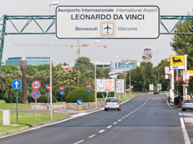
If the same driver(for example driver no. 30 was in these two spots within a 30min window frame, we can label it as a journey and extract the data points).
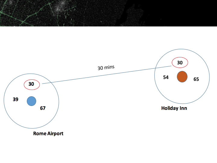
Using this hack, we extracted several different paths. Sometimes the extracted paths were taking longer than an hour. we can imagine a traffic jam could be causing this but we filter anything longer than 2.5 hours.
Mobility intelligence and Activity Analysis:
One of our goals in this project was to discover interesting cases of work ethics among the drivers. As most of the taxi fare systems are based on trip distance we can assume that in order to maximize the revenue, a taxi driver may not always take the shortest path. This means, after picking up a customer at origin zone, taxi will not move to the customer’s destination zone via the shortest path. Now sometimes there could be traffic jams and intelligent drivers could find alternate routes which are equally good, in which case. But detection of fraudulent behaviour assumes that in normal circumstances average trip should looks quit different from the optimal route should be flagged for further investigation.
We therefore need a method that can uncover the difference in taxi driver performance based on when and where they operate, routes they pick in order to reveal the differences in decisions made. We use the routes takes by the top drivers as our baseline and compare it to the low performing ones.
To compare the paths of taxi drivers we can use the VFractal approach, proposed by Nams [1][2]. This lets us to quantify tortuosity of movement paths and to compare how top and ordinary drivers operate on different spatial scales at different time. Using this approach we can can reveal driver fraudulent behaviour and their mobility intelligence.
How does it work? well, VFractal considers a movement path to be a series of turning angles for each scale. Vfractal Analysis takes in a path and returns a fractal value ranging from 1 to 2. A higher number(>1.5) represents a tortuous movement path. For each V formed by turning angle, various statistics are calculated, and then D is estimated from the mean of these statistics over the whole path.
Following equation gives an estimate of D for the V formed by one pair of steps[1]:
$$D=\frac{\log (2)}{\log \left(\frac{N e t}{s}\right)}=\frac{\theta}{1+\log _{2}(\cos \theta+1)}$$
where, s is size of one step, Net is the net distance from start of the first step to the end of the second step, and θ is the turning angle between the two steps
To estimate D for the whole path we calculate for D for each V, and then find the mean D for the whole path.
Results:
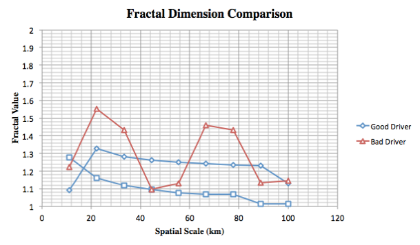
In the plot above we compare Vfractal values of three different routes taken by three different drivers(extracted in the previous step). The higher values(closer to 2.0) indicate a more torturous path, which means the driver didn’t take the most direct route even though it existed. We repeated the process for several other extracted paths and noticed a similar pattern. The results of our analysis show that taxi drivers may not always take the most optimal route. Moreover, we noticed that Taxi drivers tend to exhibit different behaviour on longer trips, as the incentives change. In particular we noticed that for a longer trip even the most top drivers(with respect to distance travelled) tend to take longer routes.
Conclusion:
In this project we used the rome taxi dataset to analyse pattern movement of taxi drivers. Analysis of this sort can yield various insights for planning bureaus, city planners and transportation analysis etc. After initial exploration and cleaning of data we extracted various routes and then Fractal analysis was employed to quantify tortuosity of movement paths in order to explore how top and ordinary drivers operate on different spatial scales at different times, where the primary focus is to reveal top driver mobility intelligence. Based on our results we can conclude that taxi drivers indeed sometimes try to maximize their income using unethical ways. Moreover, its interesting to see how taxi’ drivers intelligence can be learned from a large number of historical data.
Future work: One of the improvements that can made to this work is registering the extracted paths with the underlying road network to get more accurate comparison of paths. We also aim to perform the same analysis based on varying trip length. You can find the code on github:
References:
[1] http://www.igi-global.com/chapter/revealing-taxi-driver-mobility-intelligence/42393
[2] The VFractal: a new estimator for fractal dimension of animal movement paths http://link.springer.com/article/10.1007/BF02059856#page-1
[3] Big Trajectory Data: A Survey of Applications and Services

